Analyses of the light quantum system for Yang-Mills field.

In this article Yang-Mills field is deduced only by mechanics principles (The law of conservation of matter and Newton’s law) in light quantum system. It is shown that non-Abelian gauge Yang-Mills field of particles is essentially a mechanical process of the light quantum system. For a particle (point charge) or a complex particle, when the discussing region is farther from the center of a particle, the field round the particle is the electromagnetic field. When the discussing region is not farther from the center of the particle to consider that the distributing equipotential surfaces are curved surfaces, we must substitute the covariant derivative for the derivative in the mechanics laws (The law of conservation of matter and Newton law), so the field around the particle is the Yang-Mills field.

In this paper, the four-dimension gauge field intensity and the four-dimension gauge field potential, and other concepts are based on the oscillating energy and momentum of the light quantum system. The established processes are broke away from the Coulomb's law and the Ampere ring road law etc., which are the macroscopic experiment laws. Further proof the fact that particles are composed of the light quantum system. The oscillations of the light quantum system are the basis for forming fields.

Set up a relatively static rectangular coordinates system  to the particle, the origin  is the center of the particle.  is in the space measuring with curved metric.

Orthogonal main curvature line network and surface normal can be selected. The distributing equipotential surfaces in  can be represented as:

. ，， are the curvilinear coordinate parameters in the space measuring with curved metric. According to the principle of the infinitesimal geometry, we can choice ，, as the orthogonal main curvature network and surface normal， is the normal of the surface. These curvilinear

 coordinates can correspond to the rectangular coordinates by a rotation transformation.

In the coordinates system we take a small area round a point . In the small area ，To regardless of the higher infinitesimal can get the system of equations:

 (The law of conservation of matter),  

 (Newton’s law). 

is shown as the density of the light quantum of particlein the area ,  is shown as the three-dimensional vibration velocity.  is the stress on the light quantum in the area . Takeare external force, acted to the light quantum system in the small region.  are the outward action around the particle due

 to the vibration of light quantum system of the particle. There is no other field of force in the space around the particle.  just is the outward electric field of the particle.

Take , form this can get:

，.

The distributing equipotential surfaces are curved surfaces, the direction of the basis vector of the coordinate system varies at each point on the distribution surface.We must substitute the covariant derivative for the derivative. After substituting the covariant derivative for the derivative, the mechanics equations

 can be expressed as: .

is shown as the covariant derivative. .

Among them the subscripts  are corresponding to the physical quantity in rectangular coordinate parameters,  are corresponding to the physical

 quantity in curved coordinate parameters. These provisions shall also be applied below.

Isotropy, in establishing a rectangular coordinates system , we can choose the coordinate axis as the principal axis. When ,，When

，.

Then the stress equation in the rectangular coordinate system is:

.

The transformation from the rectangular coordinate system to the curvilinear coordinate system is:

, .

Now we are talking about a non-Abelian field. According to the theory of color dynamics, there are several chromatic symmetry states for ，，

 of each component.  The anticommutorlie matrix of Lie group is represented by. . . represents the indicator of color

symmetry state. For the non-Abelian field, the gauge field potential will change from，.      

   The stress equation in the rectangular coordinate system is:    

———。

  Namely ————

 Multiply both sides of  on the left by,

 gets:

, same material and isotropic, supposes the proportionality coefficient is ， That is  in it, thus can get:

_.

The operators，，， in the equation act on the four-dimensional components of the stress field and also act on the corresponding basis vectors.。

 is the state function of the particle,  andall are corresponding to the density of the light quantum of the particle, , there are no other factors involved,

after to substitutes forcan get：_.

It has been found in the above article: << Symmetric equations of the light quantum systems.>>: .

But we should think about replacing derivatives with covariant

derivatives, the sample we get:.

 From this we can get:

.

Among them, is the magnetic quantum number, which

corresponds to the charge.

We have seen above:

———

Multiply both sides of on the left by,

gets: .

Define, namely, ,.

This is：，. Substitute these relations into the equation , and if plug in ，

get： .        A free particle has a four dimensional energy tensor and a four dimensional state

 function,  The energy tensor have the same vibration frequency and phase as the state function, so we can think.

We have substituted forabove, imitate to substitute  for, we can substituted for, and it can be argued that. Let’s substitute for

, get: .

This expression is compared to the expression above:

，，get：

………………（1）,     in the same way:

………………（2）,

………………（3）,        Plus equation above:

.

Let’s do the following: . That is:

 , 

namely：.      From the matrix relationship  we get the three dimensional vector,

，we can be deduced：.is the gradient.

It has been decided above: ，

Is derived: ,  namely, , .     

Multiply both sides of  by, gets: ……………，

 Multiply both sides of  by, ，gets:

.

Reference is obtained:

-_,It has been deduced above .    

_， namely .    

In the same way：

. 

Plus equation above:

.

These series of four equations  are called series of equation . The matrix relation  is established by referring to the series of equation:

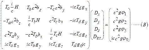
Assuming that , The equivalence for series of equation  and matrix relation  can be proved.（see <<appendix>>）

The fourth equation in the series of equation : ，

 According to the above law of conservation of matte：，For a stable system with no outside fields around it ，

，

From this can get: .

 Find the particular solution of the series of homogeneous

 equation，the matrix relation becomes the matrix relation：

 ,

Multiply both sides of on the left by, gets:

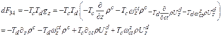
Define the matrix relationships：

This leads to the matrix relationship ：

Obtained from the above:

Obtained from the above:, ,

.

。

The unit of measure  at any point  in a rectangular coordinate system is measured by the curved metric, the length of  varies from position to position, but its direction remains the same.

.

, 

The same .

,  .

. Contrast formula

 and as described above can get: , and .

In the space measured by the curved metric:

_. The subscript “”indicates the physical quantity of the flat space,

The subscript “”or omit subscript indicates the physical quantity of the curved space,

Why do we put  here? Because the point  is any point on the surface, is just a starting point of , and. And because of isotropy, we can choose

 the coordinate axis as the principal axis when we build the coordinate system.  can be considered the same in flat space, and it doesn’t matter what is worth it.

 Isotropy, and the coordinate axis can be chosen as the principal axis when establishing the coordinate system. Which makes

 in the plane space.  Isotropy, can be expressed as a constant.  Let’s set. Except for physical units can be made

. We are going to plug ，，and  in what we have got all the formulas. Then get: , .

.  

On the other hand, in curved line coordinates, is

a four-dimensional tensor,  is the component of a tensor, It should be a vector. The length and direction of the basis vector of

 varies with the position of point.

Derivatives must be replaced by covariant derivatives in coordinate systems,we have to figure out the connection that corresponds to . On the

 surface of the light quantum system, according to differential geometry:

,

.

We can get connection from these:,

, . The vector is  in rectangular coordinates, . The vector is  in curved coordinates,

. The transformation from a rectangular coordinate system to a curved coordinate system is:

. , , ..

.

The transformation from a rectangular coordinate system to a curved coordinate system for velocity is: .

,

In rectangular Coordinate system.

The transformation from a rectangular coordinate system to a curved coordinate system is:

.

All of this says that on surface if we take a rectangular coordinate system we have .

If we take a curved coordinate system we have:

According to differential geometry, in the rectangular coordinate system, the curvature 2-basic form is expressed as

.

In the curved coordinate system, the curvature 2-basic form is expressed as.

These definitions of differential geometry are in perfect agreement with the results obtained except that differed by applying the coefficients of

 chromodynamics 、. In the Yang –Myers field, is the gauge field intensity  on the distribution surface. And connection is the gauge field

 potential. The curvature 2-basic form of the surface corresponds to the gauge field intensity_. This is an important idea of gauge fields.

Go back to the matrix relation ：

.

But in the tradition, so-called the field of a particle at a point, it is the force of the particle as a whole ( from the center to  ) on the external

 particle as a whole at point ( from the center  to ). The charge density of particle  is concentrated at point . The charge density of external

 particle  is concentrated at point too.                                             Multiply the right-hand side of the matrix relation  by  and , and

double integrate in the region , take the average of the time period:

.   

is the charge quantum number of .

  According to the paper《Analyses of the light quantum system for the electromagnetic field tensor.》, are the force of the particleon outer space at

point. For particles at rest or in motion, the force exerted on the outside caused by oscillation of the light quantum system of the particle just is the

 force of electromagnetic field.  just are the electric field of force. ，，are the magnetic force outside. In this paper, covariant derivative is always

used to replace derivative, so these arguments are also applicable to The Yaung- Myers field.

Multiply the left-hand side of the matrix relation  by  and , and double integrate in the region , take the average of the time period,

The integral of 、、 are denoted by, .  is the electric field of particle  acting on point. The integral of 、

、 is denoted by, , The strength of the stress field is the magnetic induction,  is the external magnetic field

induced by particle at point .

In this paper, covariant derivative is always used to replace derivative, so

 is the electric field component of the gauge field strength of Young-Mills when the particle is not affected by other effects.  is the magnetic field

 component of the gauge field strength of Young-Mills. Also can say: multiply the left-hand side of the matrix relation  by  and , and double

 integrate in the region  . After the integration, represents the external action field  and the rotational stress field of particle  at point .

If the quantum numberis defined as the quantity of charge,

，，，respectively represent the current density and charge density at point , then the matrix  relation is

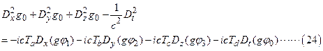
 obtained:

This is the Einstein electromagnetic tensor matrix in the gauge field.

It is exactly the same as Einsten’s electromagnetic tensor matrix:  .   

《appendix》 To prove the matrix relation  is equivalence with the series of equation:

The matrix relation : ，We from the matrix relationcan get that matrix relation ：

。

Multiply both sides of on the left by：

.    That is

. 

 From the above:

Multiply both sides of on the left by：

The previous definition are：, namely , ,. 

From these get：

 .

Namely ,

In the same way：. 

    Combined with equation : .

These four equations (21)——（24）are the result of identity transformation from matrix relations , and these four equations (21)——（24）are exactly the same with the equations （11）——（14）.Therefore, matrix relations are completely equivalent to system of equations.

Introduction and Contents 引言和目录