In-depth analysis of the curvature of general relativity

               ——Metric transformation function(1)

Einstein’s general theory of relativity holds that the “physical space” which describes physical phenomena, should be determined by the distribution of matter in space. This is a leap in the understanding of space. General relativity says that space under certain conditions is curved. The representation of space should replace Euclidean geometry with Riemannian geometry. In any 4-dimensional coordinate system of space, a space is flat space if the metric

 tensor is a constant and the curvature tensor is. A space is curvature space if the metric tensor is not constant always, and the

curvature tensor is. Corresponding to this, there are two kind of metric for two kinds of space. These are flatness metric and the curvature metric. The readings of physical quantities are related to the metric of spade. We have established two kinds of metric, use both the readings obtained by measuring with these two kinds of metric can be describe the physical quantity of two spaces respectively, namely flat space and curved space. But these are only mathematical arguments and we should discuss them in a physical sense.

Physical space is a material space and distribution of matter is not uniform. The distribution of matter varies with its position in space. So the metric of physical space has to be related to the distribution of matter.

So-called “flat space” is The Borroglie space, it actually a kind of imaginary space. The“flat metric” is a unit of measure assumed to be constant for

 the speed of light. The speed of light is assumed to be constant, whether in vacuum or where matter is densely distributed. If the speed of light is assumed to be constant in matter space, then the unit of length varies with the density of matter. The “flat metric” is a variable unit of measurement.

 In flat space, since the speed of light is assumed to be constant , the density of matter is assumed to be constant. If we measure the density by the flat

metric, it’s always.The subscript “f” represents the flat space. Measured by this metric, the free particle would be a train of plane waves. The most

 fundamental principle of quantum mechanics, Borroglie hypothesis, can be established. Using as a variable unit of measure in flat space. The subscript is shown as the reading of physical quantity measured in unit of measure of the flat metric, such as velocity, density of matter,……

The ‘curved space’ is the Einstein space, the space we’re in. The curved metric is always defined as a unit of measurement in each coordinate system of

 relative motion by the convention that the speed of light in vacuum is constant. Using this matric, the speed of light in medium is less than , even if it’s much less than , and if the light is in very dense material, the length of the units of metric will always be the same. In curved space, the speed of light varies with the density of matter, but the length of units of metric is always the same. The ‘kilogram, meter, and second’ that we use is this series

 of units. Use as a uniform invariant unit of measure in curved space, the subscript is shown as the reading of a physical quantity measured in units of metric by the curved metric. Such as the velocity,the density of matter, ……

Both the flat metric and the curved metric can be used as units of metric for the same substance, so there must be a functional relationship between

 them. Let’s express this function in terms of. That is. The reading of a physical quantity is inversely proportional to the length of

 the unit of metric. According to the above provisions, there are the radius , the length, ，the velocity

，，The surface density  ， , the volume density ， ……… This will

 be stated below and in other articles on the site.

Flat space and curved space are not two different kinds of space, it just that we measure it with two metric and then get two different readings. And there is a definite functional relationship between these two readings.

Now, the reason why we define flat space and curved space in this way is because we can agree on the definition and content of general relativity

Whether we use the flat metric or the curved metric the speed of light in vacuum is always,when, namely . For a

 particle ，When，，. .

When a particle is on a compound particle or in the field, the metric transformation function is . “” will be discussed in detail in the following articles.

How do we derive from its definition and how do we derive from these two definitions of the metric?.  Let’s start with an “independence

 principle”. There is such a fact in the field: In the absence of fission, each particle has its own unit of flat measure and metric transformation function. The intrinsic units of measure and metric transformation function for each particle remain constant in the field or around

 other particles. In the field or around other particles, if we use the intrinsic unit of metric of the particle and the metric transformation function

to measure, the result is: The particle remains as it was when it was isolated, not affected by the presence of other field or other particles. That is

 to say, in the case of no fission, if each particle is measured by its own unit of metric and the metric transformation function, its light quantum is always distributed and moving on the equipotential surface of its original isolated state, the distribution of the light quantum remains the

 same. Particles remain relatively independent. However, two particles can also be regarded as a composite. The light quantum system of two particles

 constitutes the light quantum system of compound particle. In this case, the light quantum system as composite particles will be distributed and

 moving on the equipotential plane of the compound particle. Measured in and of the compound particle, the compound particle forms a

 series of plane waves in space.

How can we derive according to the definition of and the above definition of two kinds of metric?

As shown in figure (1), the coordinate is called system for short. , are two free particles. is their composite particle. In series, is a

 point in the plane, it also is on an intersected curve of the distribution of surface of these two particles, . The coordinates of this point is

. This point is on the axis, . The pointis on the axis, The coordinates of point are. , lie on the axis of the

 plane, they corresponds to two particle, separately.

, are on the plane.is the normal line passing point on the distributing surface of light quantum of the first particle. is the

 normal line passing point on the distributing surface of light quantum of the second particle. is the radius of curvature of the normal

 transversals of equipotential surface of the first particle. is the radius of curvature of the normal transversals of equipotential surface of the second

 particle. That is to say , are the curvature centers of the normal transversals of the distribution surfaces of light quantum of two particles

 respectively. ，, that is point is the midpoint of .

On the plane , ， .  , are the tangents of the normal transversals of the two equipotential surfaces of the light quantum

 respectively So the light quantum of two particles, at , are moving in the and respectively. (Clockwise direction). is on the plane , it is

 across , and it is the tangent line of the distributed equipotential surface of the light quantum of the composite particle. As a compound particle, the

 light quantum will move in the opposite direction of at.  Let’s draw the straight line perpendicular to, on the plane. is the

 normal of the distributed equipotential surface of the light quantum of the composite particle. is the radius of curvature of normal transversal of

 equipotential surface of compound particle. Point doesn’t have to be on the axis.

, , , , 。

，，. ,, . , pointis on the axis.

As,, .  

In the triangle, let ，, .

In the triangle, let ， , .

，.

For the first particle, the light quantum is moving in thedirection.  For the second particle , the light quantum is moving in the direction. The

light quantum of composite particles move in the direction, after the collision at point, the sum of the momentum in the direction is equal to zero.

, ，the sum of the momentum in the direction is equal to zero.

.They are readings measured in the units of the curved metric.

For,, the light quantum are distributed on the tangent surface of the distributed surface, they are move in each direction in equal probability.

Their velocity are all equiprobability vector, It is only a small fraction in the direction.                                    

With centerand radius, make a sphere through point . And also makes a solid angle element with as the vertex, as the radius,

it intersects the sphere at. , is the radius vector. is the apex angle of solid angle. Let the width at the

intersecting planeofis.

Let is the surface area of the volume element occupied by the light quantum of the particle moving along the plane..

is the angle between two radio from the center of the sphere to two endpoints of .  

Let is a solid angle with vertex and surface area of the volume element. .

,.  should be the directional probability of the light quantum of the particle moving

along the direction. The directional probability of the light quantum of the particle moving along the direction is .

Similarly, With centerand radius, make a sphere through point , and with radius as a solid angle element, and make.

is the vertex angle element of solid angle, intersects the sphere at , the width where meets is . ,

.

Let is the surface area of the volume element occupied by the light quantum of the particle moving along the plane.

, is the angle between two radio from the center of the sphere to two endpoints of.

The same analysis can be obtained. The directional probability of the light quantum of the particle moving along the direction is.

.

We have taken, so we have . The corresponding angle of the corresponding string is,

. In fact, the light quantum in , cannot all be hit in the positively direction. Only the light

 quantum mass point of two particles in, is positively collided in the .  , are only within a small part

 of , . Therefore, in，, the probability of positive collision between the light quantum mass point of

 two particle along the direction at the time interval of is ， . The analysis is as follows: As shown in the figure 2.

Located at point ,， are the effective diameters of the light quantum mass point of the two particles, respectively. At time, there is a pair of

light quantum mass point handling positive collisions in point. At time, the distance traveled by the first light quantum mass point is, the distance

traveled by the second light quantum mass point is .

In the period of , the light quantum mass point with the effective diameter of can have a positive collision with the light quantum mass point with the effective diameter of . In the period, the light quantum mass point with the effective diameter of to the light quantum mass point with the effective diameter of can positive collisions each other within the distance of, which has a productive area. In the same way, in the time period , the light quantum mass point with the effective diameter of to the light quantum mass point with the effective diameter of can positive collisions each other within the distance of, which has a productive area . While，， .  The

 resulting is . For two light quantum there are. The probability of a positive collision are ，

 respectively. While，, it means on the distributing surface of the light quantum, two light quantum mass points moving in the

 direction pass point have the same probability of positive collision in the time interval . We have got above

. Let’s consider the directional probability ,  . In addition, the probability of positive collision

between two light quantum mass points along a certain direction in a certain time interval for， should also be and

respectively. So if there are “n” time collisions in this region during this period of time, then the probability of positive collision are，

 respectively.  After the reduction.  

 . ，. The density of the light quantum mass points in the volume element is

. For the curved metric, . We can get from these: ………（2）.

               Go back to figure 1: , , , . is on

 the opposite extension of .

，，. ,,           

, point M is on the axis. when,, . In the triangle, let,,

. Let, is tangent to the equipotential surface ,.

.

.

.

, . , .

It can be obtained from formula （2）:,.

。

.

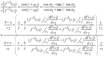i.e 。

The resulting：。 is an increasing function, Let’s。 .  . Let ， For each

 normal transversal that passes through point on the equipotential plane of the particle, the metric transformation function is .

is the normal curvature of the normal transversal on the surface of light quantum of the particle. . Take the average of the normal curvature of

 the normal transversal, get.. , are the principal curvatures of the curves , on the distribution curved

 surface respectively. Because the equipotential distribution surface of light quantum is minimal surface, . That’s we can get: ,

, .

 is the Gaussian curvature at point on the surface of light quantum of the particle, , . The average metric conversion function

 for point on the distribution surface of light quantum of a particle is .. For all particles “”is a common number,

 probably related to Planck’s constant. is a integral constant, which is determined by the initial conditions of the differential equation. The following

 article will discuss it in detail.

Introduction and Contents 引言和目录